Future projections
Recent additions to this website have added trend calculations to project future values of temperatures and other metrics. They are found in:
- The temperature trend on the location dashboard, and as a sortable column on the locations list. It reports a linear rate of change per decade over the last 30 years, or, if that is not a significant trend, over the full range of years.
- The recent observations panel on every location page. It reports a linear rate of change per decade for temperature and rainfall.
- Charts that can have up to three trend lines per series.
- Built-in presets for charts - a per-location temperature trend, and a global CO₂ trend.
Trend calculations are offered via two similar pieces of maths:
- Linear regression: the straight line through a set of points.
- Quadratic regression: an approach that allows the line to bend into a curve.
This post explains how they're calculated.
Where to find trends
Location dashboard
Each location's dashboard shows a single headline temperature trend that is:
- the rate of change per decade over the last 30 years when that is statistically significant, otherwise over the full record
Click the temperature trend for details. The popup lists three windows (the full period, the last 30 years and the first half of the data). It says whether each is significant and gives its p-value. Its "About trends" panel then breaks each window down into the statistics behind it, using that location's own numbers, and lets you download the yearly data. The same headline rate is a sortable Temperature trend column on the locations list, so you can rank locations from fastest warming to slowest. Locations with no significant trend will not display a value.
Trend tab in recent observations
The Trend tab in Recent Observations fits a straight line to a metric's yearly history and reports the slope as a rate per decade, for the same three overlapping windows: the full period of record, the last 30 years, and the first half of the record. Comparing the three is a quick check for acceleration - if the last-30-years rate is steeper than the early-period rate, the metric isn't just trending, it's trending faster than it used to. As on the dashboard, a trend only gets reported at all once it clears a statistical significance bar; short of that, the tile plainly says "No significant trend" rather than printing a number that isn't reliably different from noise. There's a much fuller explanation of all of this, worked example included, behind the "About trends" link on that tab.
Charts
Charts go further. Any chart series can carry up to three trend lines, each independently configured: linear, quadratic, or cubic; fitted to the full record, the last 30 years, or the first half; and projected forward by a fixed number of years or out to a target year.
We support more than one trend per series, because a trend line is a possible future, not a certainty - showing three different fits side by side is a better answer to "where is this headed?" than picking one and presenting it as the answer.
Two chart presets use this. Temperature + trend, on every location page, fits both a linear and a quadratic trend to the full temperature record and projects 50 years out. Atmospheric CO₂ vs emissions, on the global page, is the one we'll spend the second half of this post on.
Linear regression: a straight line through the data
A trend line here is an ordinary least-squares linear regression.
To understand how it's calculated, picture each year as a point: x is the year, y is that year's value. The slope, β, comes from:
β = Σ(x − x̄)(y − ȳ) / Σ(x − x̄)²
- Σ is the mathematical symbol for sum: perform the calculation for each year, then add all the results together.
- x̄ and ȳ are the average year and average value across the record.
For every year, take how far that year is from the average year, and how far its value is from the average value, and multiply the two together; add that up across every year for the sum on top. The sum on the bottom does the same thing with just the years, squared. Divide one by the other and the result is the slope - how much the fitted line rises for every extra year.
Worked example
Take the annual mean CO₂ concentration measured at Mauna Loa for 1960 to 1969, in parts per million, rounded to the nearest whole number:
| Year | ppm |
|---|---|
| 1960 | 317 |
| 1961 | 318 |
| 1962 | 318 |
| 1963 | 319 |
| 1964 | 320 |
| 1965 | 320 |
| 1966 | 321 |
| 1967 | 322 |
| 1968 | 323 |
| 1969 | 325 |
The average year is 1964.5 and the average concentration is 320.3 ppm. The regression finds the one straight line that best fits all ten points at once.
| Year (x) | ppm (y) | x − x̄ | y − ȳ | (x−x̄)(y−ȳ) | (x−x̄)² |
|---|---|---|---|---|---|
| 1960 | 317 | −4.5 | −3.3 | 14.9 | 20.25 |
| 1961 | 318 | −3.5 | −2.3 | 8.1 | 12.25 |
| 1962 | 318 | −2.5 | −2.3 | 5.8 | 6.25 |
| 1963 | 319 | −1.5 | −1.3 | 2.0 | 2.25 |
| 1964 | 320 | −0.5 | −0.3 | 0.2 | 0.25 |
| 1965 | 320 | 0.5 | −0.3 | −0.2 | 0.25 |
| 1966 | 321 | 1.5 | 0.7 | 1.0 | 2.25 |
| 1967 | 322 | 2.5 | 1.7 | 4.2 | 6.25 |
| 1968 | 323 | 3.5 | 2.7 | 9.4 | 12.25 |
| 1969 | 325 | 4.5 | 4.7 | 21.1 | 20.25 |
| Sum | 66.5 | 82.5 |
The slope is the sum on top divided by the sum on the bottom: 66.5 ÷ 82.5 ≈ 0.8 ppm per year.
Now the most recent complete decade on record, 2016 to 2025:
| Year | ppm |
|---|---|
| 2016 | 404 |
| 2017 | 407 |
| 2018 | 409 |
| 2019 | 412 |
| 2020 | 414 |
| 2021 | 416 |
| 2022 | 419 |
| 2023 | 421 |
| 2024 | 425 |
| 2025 | 427 |
Same method, mean year 2020.5 and mean concentration 415.4 ppm, gives Σ(x−x̄)(y−ȳ) = 208.0 and Σ(x−x̄)² = 82.5 - the spread of years is identical. The slope is 208.0 ÷ 82.5 ≈ 2.5 ppm per year.
The straight-line rate more than tripled between the 1960s and 2020s: 0.8 ppm per year vs 2.5 ppm per year. That's the limit of ordinary least squares: it forces one constant rate of change onto whatever window you feed it. Recent Observations shows three overlapping windows for this reason, and charts let you stack multiple trend lines: comparing them is how you notice a record that isn't behaving in a straight line at all.
Quadratic regression: letting the line bend
The full equation of the straight line is:
y = β₀ + β₁(x − x̄)
- β₀ is ȳ (described above) - the average of the values
- β₁ is the slope β calculated above
The line goes through the average year at the average value, and rises β₁ for every year after that. A quadratic regression adds one more term:
y = β₀ + β₁(x − x̄) + β₂(x − x̄)²
The new term lets the line bend. If β₂ is positive, the curve is a gentle upward bow that gets steeper as time goes on. If it's negative, the curve flattens out. If it's zero, that's a straight line.
The steps are harder to follow, although the maths is similar. Call the new quantity z = (x − x̄)², the squared distance of each year from the middle year. That's the same number that's already in the last column of the linear table. Because the years run without gaps and are centred on the middle year, the two halves of the record pair up: the first year and the last year are the same distance from the middle, so they get the same z. That means z only measures how far a year is from the middle, not which side it's on. The straight-line part (x − x̄) only measures which side and by how much. The two don't overlap, so each coefficient can be worked out separately with the same slope formula from the linear section:
- β₁ is the slope of y against (x − x̄). This is exactly the straight-line calculation.
- β₂ is the slope of y against z. It's the same formula again, with z in place of x: β₂ = Σ(z − z̄)(y − ȳ) / Σ(z − z̄)².
- β₀ = ȳ − β₂·z̄. This is the one change from the straight line, and it's needed because z̄ isn't zero.
It is one extra table and one extra division. That shortcut depends on the years being evenly spaced with no gaps. If some years are missing, the three coefficients have to be found together by solving three simultaneous equations (the "normal equations"). That's what ClimateExplorer does in general, and for a gap-free record like this one the answer is identical.
How fast is CO₂ accelerating?
For a quadratic regression of atmospheric CO₂, this time we use the whole record: every complete year from 1959 to 2025, which is 67 years. The annual means are rounded to the nearest whole ppm, as in the linear example. The middle year is x̄ = 1992 and the average concentration is ȳ = 24,205 ÷ 67 ≈ 361.27 ppm.
First, the straight-line part. This table has the same columns as the linear tables above, with most of the 67 rows left out:
| Year (x) | ppm (y) | x − x̄ | y − ȳ | (x−x̄)(y−ȳ) | (x−x̄)² |
|---|---|---|---|---|---|
| 1959 | 316 | −33 | −45.27 | 1,493.9 | 1,089 |
| 1960 | 317 | −32 | −44.27 | 1,416.6 | 1,024 |
| ⋮ | |||||
| 1991 | 356 | −1 | −5.27 | 5.3 | 1 |
| 1992 | 357 | 0 | −4.27 | 0.0 | 0 |
| 1993 | 357 | 1 | −4.27 | −4.3 | 1 |
| ⋮ | |||||
| 2024 | 425 | 32 | 63.73 | 2,039.4 | 1,024 |
| 2025 | 427 | 33 | 65.73 | 2,169.1 | 1,089 |
| Sum | 41,936 | 25,058 |
β₁ = 41,936 ÷ 25,058 ≈ 1.674 ppm per year. That's the straight-line slope for the whole record, and it's also the curve's rate of change at the middle year, 1992.
Next, the bend. Take the last column above as z. Its average is z̄ = 25,058 ÷ 67 = 374. Then repeat the method with z in place of x:
| Year | z = (x−x̄)² | z − z̄ | y − ȳ | (z−z̄)(y−ȳ) | (z−z̄)² |
|---|---|---|---|---|---|
| 1959 | 1,089 | 715 | −45.27 | −32,367.1 | 511,225 |
| 1960 | 1,024 | 650 | −44.27 | −28,774.6 | 422,500 |
| ⋮ | |||||
| 1991 | 1 | −373 | −5.27 | 1,965.2 | 139,129 |
| 1992 | 0 | −374 | −4.27 | 1,596.5 | 139,876 |
| 1993 | 1 | −373 | −4.27 | 1,592.2 | 139,129 |
| ⋮ | |||||
| 2024 | 1,024 | 650 | 63.73 | 41,425.4 | 422,500 |
| 2025 | 1,089 | 715 | 65.73 | 46,997.9 | 511,225 |
| Sum | 100,702 | 7,492,342 |
Look at 1959 and 2025: they have the same z, but the 2025 CO₂ reading is far above the average concentration (ȳ) while the 1959 reading is far below it. Most of the bend comes from the ends of the record. The 1959 reading is below ȳ by a bit less than a straight line would predict, and the 2025 reading is above ȳ by more than a straight line would predict.
β₂ = 100,702 ÷ 7,492,342 ≈ 0.01344, and β₀ = 361.27 − 0.01344 × 374 ≈ 356.24. The fitted curve is:
CO₂ ≈ 356.24 + 1.674(x − 1992) + 0.01344(x − 1992)²
It fits the 67 years far better than a straight line does: R² is 0.999, against 0.981 for the line.
On a curve, "the slope" is different at every point. The rate of change at any year is:
rate = β₁ + 2β₂(x − x̄) = 1.674 + 0.0269 × (year − 1992)
(To check it, work out the curve for two neighbouring years and subtract one from the other. The difference matches this formula for the point halfway between them.) Put simply, the rise in CO₂ itself goes up by about 0.027 ppm per year, every year. Over a decade, the annual rise is about 0.27 ppm per year faster:
| Year | ppm | Rate of change |
|---|---|---|
| 1965 | 320.9 | 0.9 ppm per year |
| 1975 | 331.7 | 1.2 ppm per year |
| 1985 | 345.2 | 1.5 ppm per year |
| 1995 | 361.4 | 1.8 ppm per year |
| 2005 | 380.3 | 2.0 ppm per year |
| 2015 | 401.8 | 2.3 ppm per year |
| 2025 | 426.1 | 2.6 ppm per year |
ppm is the curve's value for that year, not the measured annual mean. The two are always within 2 ppm of each other.
Interpretation
The annual increase in CO₂ has nearly tripled over 60 years, and it has increased steadily, decade after decade. The two ten-year straight lines found above, 0.8 ppm per year for the 1960s and 2.5 ppm per year for 2016-2025, are close to this curve's rate at the middle of each of those decades (0.9 and 2.4). They are two snapshots of one long, steady acceleration.
Atmospheric CO₂ builds up from fossil fuel and cement emissions, and those emissions have increased over time. The amount added to the atmosphere each year is larger than the year before. That's a rate of change that is itself changing. A straight line can't represent that at all, and a quadratic is the simplest curve that can. Where ClimateExplorer reports a single number for a curved trend, it gives the rate at the most recent year, like the 2025 row above. The CO₂ preset described next fits its quadratic to the last 30 years rather than the whole record.
The CO₂ preset, and a real discrepancy
The Atmospheric CO₂ vs emissions preset plots two series together: CO₂ measured in the atmosphere at Mauna Loa (brown), and reported global CO₂ emissions from the Global Carbon Project (black). The atmosphere series carries a quadratic trend fitted to its last 30 years of data, projected out to 2100; the emissions series carries two, one over the full record and one over its last 30 years, both projected the same way.
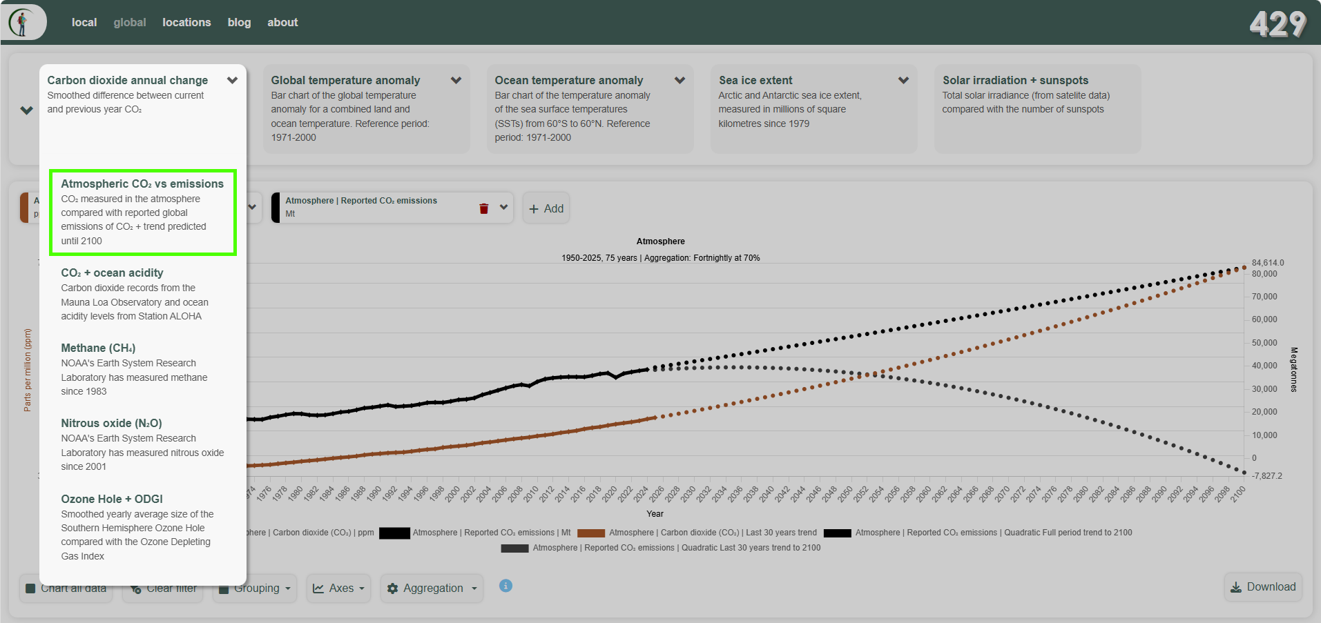
Atmospheric CO₂ (brown) and reported CO₂ emissions (black), each with a quadratic trend fitted to the last 30 years of data (ending 2025) and projected to 2100. The atmospheric trend predicts CO₂ concentrations over 730 ppm by 2100 (up from 427 ppm in 2025). The reported-emissions trend, fitted the same way, predicts emissions going negative well before then - a physical impossibility. A purely mathematical curve fit has no concept of a floor at zero, so nothing stops it projecting negative values for a quantity - emissions, or rainfall, or ice extent - that can never actually go below zero.
The two trends are saying very different things: atmospheric CO₂'s rate of increase is accelerating, and reported emissions appear to be flattening out. Those are opposite directions for numbers that we may expect to move together - more emitted should mean more measured in the atmosphere. A few reasons a gap like this can open up:
- A direct measurement versus a modelled estimate. Mauna Loa's reading is air sampled and analysed on-site. Reported national emissions are built from energy-use statistics, industrial data and modelling assumptions, and are revised for years after first publication - the most recent few years of almost any emissions inventory are its least certain, and the most likely to be revised upwards later.
- Untracked military and conflict emissions.
- UNFCCC Decision 2/CP.3, adopted at Kyoto in 1997 following lobbying by the US Department of Defense, explicitly excludes emissions from multilateral operations under the UN Charter from national totals. The Paris Agreement (2015) went further, making all military reporting voluntary; as of 2023 only Germany, the UK, the US and Norway reported any military figures.
- The IPCC's 2006 inventory guidelines (Volume 1, Chapter 8) place military fuel use under category 1.A.5 and permit aggregation for national security reasons.
- Wartime and conflict emissions receive no guidance at all.
- The Global Carbon Project's (GCP) national totals, built from the same UNFCCC-based energy statistics, inherit these gaps.
- International aviation and shipping.
- Emissions from international flights and voyages have been excluded from national inventories since the original 1994 IPCC guidelines, reaffirmed by Decision 2/CP.3. Kyoto's Article 2.2 delegated responsibility for these to ICAO (aviation) and the IMO (shipping) rather than national governments, but neither agency has established binding reduction targets comparable to national inventory obligations.
- GCP does include international bunker fuels in its global figures, reported separately from national totals, so they appear in the black series on the chart above - but no country carries them in its national target.
- Weakening sinks, not just changing sources. Atmospheric CO₂ concentration reflects the cumulative balance of all human emissions against all absorption - not just this year's. Land ecosystems and the ocean draw CO₂ down continuously from the total atmospheric stock, on timescales ranging from months (surface vegetation) to centuries (deep ocean). Historically, roughly half of all cumulative human emissions have been absorbed this way - a ratio called the airborne fraction. If those sinks are becoming less effective as the planet warms - drought-stressed forests, wildfires, marine heatwaves, shifting ocean carbon chemistry - the airborne fraction rises: a larger share of each year's emissions accumulates rather than being drawn down. That alone would show up as atmospheric CO₂ accelerating even against flat emissions.
- Natural carbon feedbacks. As temperatures rise, some natural carbon stores that were previously stable or net-absorbing have started to emit. Thawing permafrost releases CO₂ and methane from organic matter frozen since the last ice age; warming ocean surfaces, which hold less dissolved gas at higher temperatures, return CO₂ to the air. Destabilising seafloor sediments release further methane (methane hydrates). None of these sources appear in any human emissions inventory. The permafrost carbon pool alone holds roughly twice as much carbon as is currently in the atmosphere - even a small fraction mobilising over decades would register clearly at Mauna Loa.
None of that means either curve is "right" and the other "wrong" - it means a mathematical extrapolation of either one, 75 years into the future, is leaning on an assumption (today's rate of change holding indefinitely) that a 30-year window can't itself confirm. That's the same limitation the app's own trend explainer calls out for curved fits: the shorter and more recent the window, the harder that assumption has to work.
Why not cubic?
The regression tool in ClimateExplorer supports one degree beyond quadratic - a cubic fit, y = β₀ + β₁x + β₂x² + β₃x³, which can bend one way and then the other. We don't use it in either built-in preset, because the extra flexibility mostly fits noise: a cubic can match the existing years closely, but projected forward its tail swings sharply up or down, so the further out you look the less the projection means. Treat a barely-significant cubic fit with more scepticism than a barely-significant line or curve.
Checking the numbers
Every trend on a chart or in Recent Observations carries a tooltip with the underlying statistics - p-value, R², sample size - and the "About trends" panel has the same worked-through maths, using its own shorter illustrative example. On a location's dashboard, the trend popup shows each window's p-value, and its "About trends" panel shows the full statistics for that location, with the yearly data available to download.